Artificial Intelligence Nanodegree
Voice User Interfaces
Project: Speech Recognition with Neural Networks
In this notebook, some template code has already been provided for you, and you will need to implement additional functionality to successfully complete this project. You will not need to modify the included code beyond what is requested. Sections that begin with '(IMPLEMENTATION)' in the header indicate that the following blocks of code will require additional functionality which you must provide. Please be sure to read the instructions carefully!
Note: Once you have completed all of the code implementations, you need to finalize your work by exporting the Jupyter Notebook as an HTML document. Before exporting the notebook to html, all of the code cells need to have been run so that reviewers can see the final implementation and output. You can then export the notebook by using the menu above and navigating to \n", "File -> Download as -> HTML (.html). Include the finished document along with this notebook as your submission.
In addition to implementing code, there will be questions that you must answer which relate to the project and your implementation. Each section where you will answer a question is preceded by a 'Question X' header. Carefully read each question and provide thorough answers in the following text boxes that begin with 'Answer:'. Your project submission will be evaluated based on your answers to each of the questions and the implementation you provide.
Note: Code and Markdown cells can be executed using the Shift + Enter keyboard shortcut. Markdown cells can be edited by double-clicking the cell to enter edit mode.
The rubric contains optional "Stand Out Suggestions" for enhancing the project beyond the minimum requirements. If you decide to pursue the "Stand Out Suggestions", you should include the code in this Jupyter notebook.
Introduction
In this notebook, you will build a deep neural network that functions as part of an end-to-end automatic speech recognition (ASR) pipeline! Your completed pipeline will accept raw audio as input and return a predicted transcription of the spoken language. The full pipeline is summarized in the figure below.
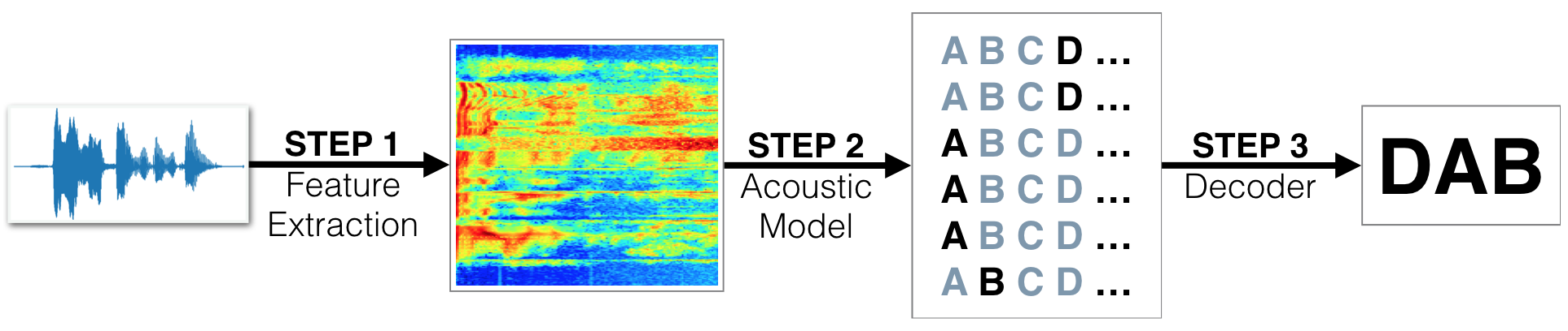
- STEP 1 is a pre-processing step that converts raw audio to one of two feature representations that are commonly used for ASR.
- STEP 2 is an acoustic model which accepts audio features as input and returns a probability distribution over all potential transcriptions. After learning about the basic types of neural networks that are often used for acoustic modeling, you will engage in your own investigations, to design your own acoustic model!
- STEP 3 in the pipeline takes the output from the acoustic model and returns a predicted transcription.
Feel free to use the links below to navigate the notebook:
- The Data
- STEP 1: Acoustic Features for Speech Recognition
- STEP 2: Deep Neural Networks for Acoustic Modeling
- Model 0: RNN
- Model 1: RNN + TimeDistributed Dense
- Model 2: CNN + RNN + TimeDistributed Dense
- Model 3: Deeper RNN + TimeDistributed Dense
- Model 4: Bidirectional RNN + TimeDistributed Dense
- Models 5+
- Compare the Models
- Final Model
- STEP 3: Obtain Predictions
The Data
We begin by investigating the dataset that will be used to train and evaluate your pipeline. LibriSpeech is a large corpus of English-read speech, designed for training and evaluating models for ASR. The dataset contains 1000 hours of speech derived from audiobooks. We will work with a small subset in this project, since larger-scale data would take a long while to train. However, after completing this project, if you are interested in exploring further, you are encouraged to work with more of the data that is provided online.
In the code cells below, you will use the vis_train_features module to visualize a training example. The supplied argument index=0 tells the module to extract the first example in the training set. (You are welcome to change index=0 to point to a different training example, if you like, but please DO NOT amend any other code in the cell.) The returned variables are:
vis_text- transcribed text (label) for the training example.vis_raw_audio- raw audio waveform for the training example.vis_mfcc_feature- mel-frequency cepstral coefficients (MFCCs) for the training example.vis_spectrogram_feature- spectrogram for the training example.vis_audio_path- the file path to the training example.
from data_generator import vis_train_features

# extract label and audio features for a single training example
vis_text, vis_raw_audio, vis_mfcc_feature, vis_spectrogram_feature, vis_audio_path = vis_train_features()
The following code cell visualizes the audio waveform for your chosen example, along with the corresponding transcript. You also have the option to play the audio in the notebook!
from IPython.display import Markdown, display
from data_generator import vis_train_features, plot_raw_audio
from IPython.display import Audio
%matplotlib inline

# plot audio signal
plot_raw_audio(vis_raw_audio)
# print length of audio signal
display(Markdown('**Shape of Audio Signal** : ' + str(vis_raw_audio.shape)))
# print transcript corresponding to audio clip
display(Markdown('**Transcript** : ' + str(vis_text)))
# play the audio file
Audio(vis_audio_path)

STEP 1: Acoustic Features for Speech Recognition
For this project, you won't use the raw audio waveform as input to your model. Instead, we provide code that first performs a pre-processing step to convert the raw audio to a feature representation that has historically proven successful for ASR models. Your acoustic model will accept the feature representation as input.
In this project, you will explore two possible feature representations. After completing the project, if you'd like to read more about deep learning architectures that can accept raw audio input, you are encouraged to explore this research paper.
Spectrograms
The first option for an audio feature representation is the spectrogram. In order to complete this project, you will not need to dig deeply into the details of how a spectrogram is calculated; but, if you are curious, the code for calculating the spectrogram was borrowed from this repository. The implementation appears in the utils.py file in your repository.
The code that we give you returns the spectrogram as a 2D tensor, where the first (vertical) dimension indexes time, and the second (horizontal) dimension indexes frequency. To speed the convergence of your algorithm, we have also normalized the spectrogram. (You can see this quickly in the visualization below by noting that the mean value hovers around zero, and most entries in the tensor assume values close to zero.)
from data_generator import plot_spectrogram_feature

# plot normalized spectrogram
plot_spectrogram_feature(vis_spectrogram_feature)
# print shape of spectrogram
display(Markdown('**Shape of Spectrogram** : ' + str(vis_spectrogram_feature.shape)))

Mel-Frequency Cepstral Coefficients (MFCCs)
The second option for an audio feature representation is MFCCs. You do not need to dig deeply into the details of how MFCCs are calculated, but if you would like more information, you are welcome to peruse the documentation of the python_speech_features Python package. Just as with the spectrogram features, the MFCCs are normalized in the supplied code.
The main idea behind MFCC features is the same as spectrogram features: at each time window, the MFCC feature yields a feature vector that characterizes the sound within the window. Note that the MFCC feature is much lower-dimensional than the spectrogram feature, which could help an acoustic model to avoid overfitting to the training dataset.
from data_generator import plot_mfcc_feature

# plot normalized MFCC
plot_mfcc_feature(vis_mfcc_feature)
# print shape of MFCC
display(Markdown('**Shape of MFCC** : ' + str(vis_mfcc_feature.shape)))

When you construct your pipeline, you will be able to choose to use either spectrogram or MFCC features. If you would like to see different implementations that make use of MFCCs and/or spectrograms, please check out the links below:
- This repository uses spectrograms.
- This repository uses MFCCs.
- This repository also uses MFCCs.
- This repository experiments with raw audio, spectrograms, and MFCCs as features.
STEP 2: Deep Neural Networks for Acoustic Modeling
In this section, you will experiment with various neural network architectures for acoustic modeling.
You will begin by training five relatively simple architectures. Model 0 is provided for you. You will write code to implement Models 1, 2, 3, and 4. If you would like to experiment further, you are welcome to create and train more models under the Models 5+ heading.
All models will be specified in the sample_models.py file. After importing the sample_models module, you will train your architectures in the notebook.
After experimenting with the five simple architectures, you will have the opportunity to compare their performance. Based on your findings, you will construct a deeper architecture that is designed to outperform all of the shallow models.
For your convenience, we have designed the notebook so that each model can be specified and trained on separate occasions. That is, say you decide to take a break from the notebook after training Model 1. Then, you need not re-execute all prior code cells in the notebook before training Model 2. You need only re-execute the code cell below, that is marked with RUN THIS CODE CELL IF YOU ARE RESUMING THE NOTEBOOK AFTER A BREAK, before transitioning to the code cells corresponding to Model 2.
#####################################################################
# RUN THIS CODE CELL IF YOU ARE RESUMING THE NOTEBOOK AFTER A BREAK #
#####################################################################

# allocate 50% of GPU memory (if you like, feel free to change this)
from keras.backend.tensorflow_backend import set_session
import tensorflow as tf
config = tf.ConfigProto()
config.gpu_options.per_process_gpu_memory_fraction = 0.5
set_session(tf.Session(config=config))

# watch for any changes in the sample_models module, and reload it automatically
%load_ext autoreload
%autoreload 2
#%reload_ext autoreload
# import NN architectures for speech recognition
from sample_models import *
# import function for training acoustic model
from train_utils import train_model
Model 0: RNN
Given their effectiveness in modeling sequential data, the first acoustic model you will use is an RNN. As shown in the figure below, the RNN we supply to you will take the time sequence of audio features as input.
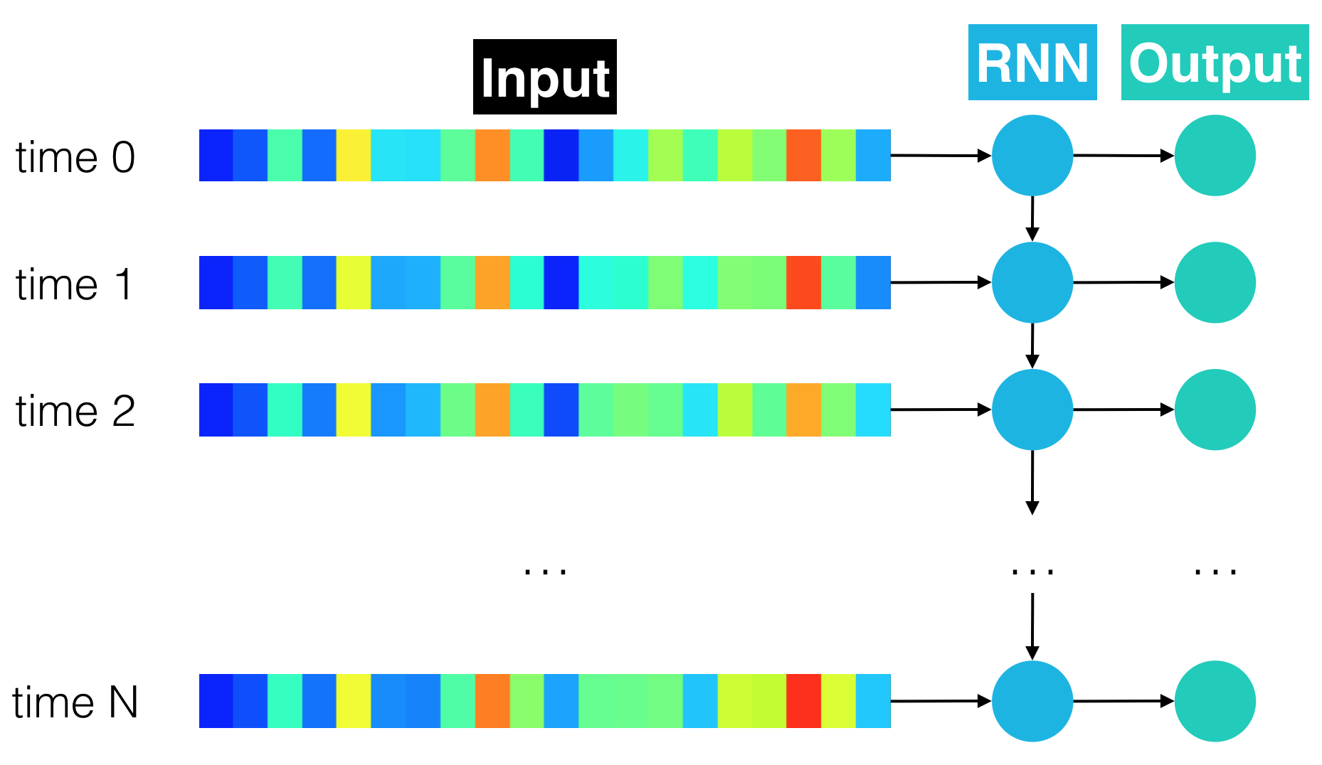
At each time step, the speaker pronounces one of 28 possible characters, including each of the 26 letters in the English alphabet, along with a space character (" "), and an apostrophe (').
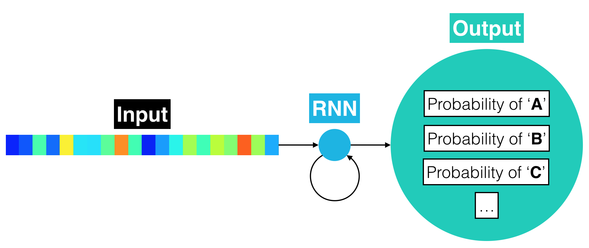
The output of the RNN at each time step is a vector of probabilities with 29 entries, where the $i$-th entry encodes the probability that the $i$-th character is spoken in the time sequence. (The extra 29th character is an empty "character" used to pad training examples within batches containing uneven lengths.) If you would like to peek under the hood at how characters are mapped to indices in the probability vector, look at the char_map.py file in the repository. The figure below shows an equivalent, rolled depiction of the RNN that shows the output layer in greater detail.
The model has already been specified for you in Keras. To import it, you need only run the code cell below.
model_0 = simple_rnn_model(input_dim=161) # change to 13 if you would like to use MFCC features
As explored in the lesson, you will train the acoustic model with the CTC loss criterion. Custom loss functions take a bit of hacking in Keras, and so we have implemented the CTC loss function for you, so that you can focus on trying out as many deep learning architectures as possible :). If you'd like to peek at the implementation details, look at the add_ctc_loss function within the train_utils.py file in the repository.
To train your architecture, you will use the train_model function within the train_utils module; it has already been imported in one of the above code cells. The train_model function takes three required arguments:
input_to_softmax- a Keras model instance.pickle_path- the name of the pickle file where the loss history will be saved.save_model_path- the name of the HDF5 file where the model will be saved.
If we have already supplied values for input_to_softmax, pickle_path, and save_model_path, please DO NOT modify these values.
There are several optional arguments that allow you to have more control over the training process. You are welcome to, but not required to, supply your own values for these arguments.
minibatch_size- the size of the minibatches that are generated while training the model (default:20).spectrogram- Boolean value dictating whether spectrogram (True) or MFCC (False) features are used for training (default:True).mfcc_dim- the size of the feature dimension to use when generating MFCC features (default:13).optimizer- the Keras optimizer used to train the model (default:SGD(lr=0.02, decay=1e-6, momentum=0.9, nesterov=True, clipnorm=5)).epochs- the number of epochs to use to train the model (default:20). If you choose to modify this parameter, make sure that it is at least 20.verbose- controls the verbosity of the training output in themodel.fit_generatormethod (default:1).sort_by_duration- Boolean value dictating whether the training and validation sets are sorted by (increasing) duration before the start of the first epoch (default:False).
The train_model function defaults to using spectrogram features; if you choose to use these features, note that the acoustic model in simple_rnn_model should have input_dim=161. Otherwise, if you choose to use MFCC features, the acoustic model should have input_dim=13.
We have chosen to use GRU units in the supplied RNN. If you would like to experiment with LSTM or SimpleRNN cells, feel free to do so here. If you change the GRU units to SimpleRNN cells in simple_rnn_model, you may notice that the loss quickly becomes undefined (nan) - you are strongly encouraged to check this for yourself! This is due to the exploding gradients problem. We have already implemented gradient clipping in your optimizer to help you avoid this issue.
IMPORTANT NOTE: If you notice that your gradient has exploded in any of the models below, feel free to explore more with gradient clipping (the clipnorm argument in your optimizer) or swap out any SimpleRNN cells for LSTM or GRU cells. You can also try restarting the kernel to restart the training process.
train_model(input_to_softmax=model_0,
            pickle_path='model_0.pickle',
            save_model_path='model_0.h5',
            spectrogram=True) # change to False if you would like to use MFCC features
(IMPLEMENTATION) Model 1: RNN + TimeDistributed Dense
Read about the TimeDistributed wrapper and the BatchNormalization layer in the Keras documentation. For your next architecture, you will add batch normalization to the recurrent layer to reduce training times. The TimeDistributed layer will be used to find more complex patterns in the dataset. The unrolled snapshot of the architecture is depicted below.
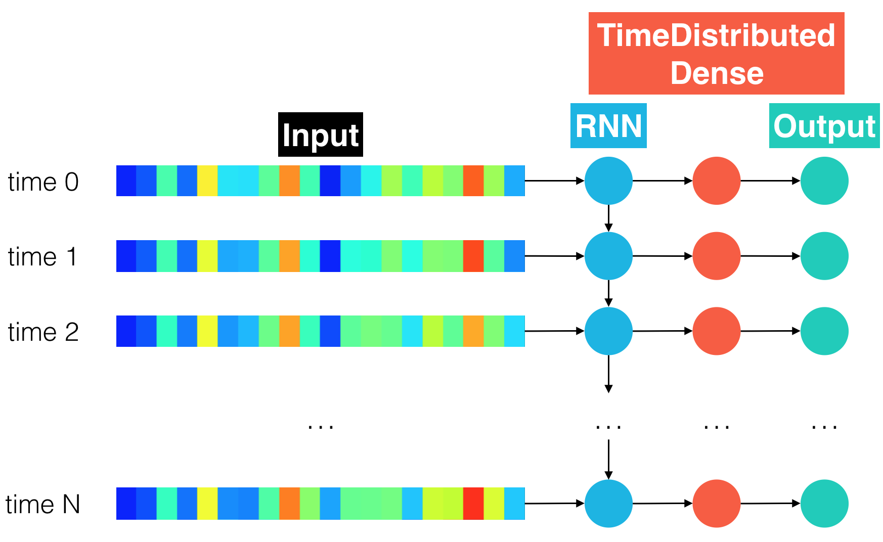
The next figure shows an equivalent, rolled depiction of the RNN that shows the (TimeDistrbuted) dense and output layers in greater detail.
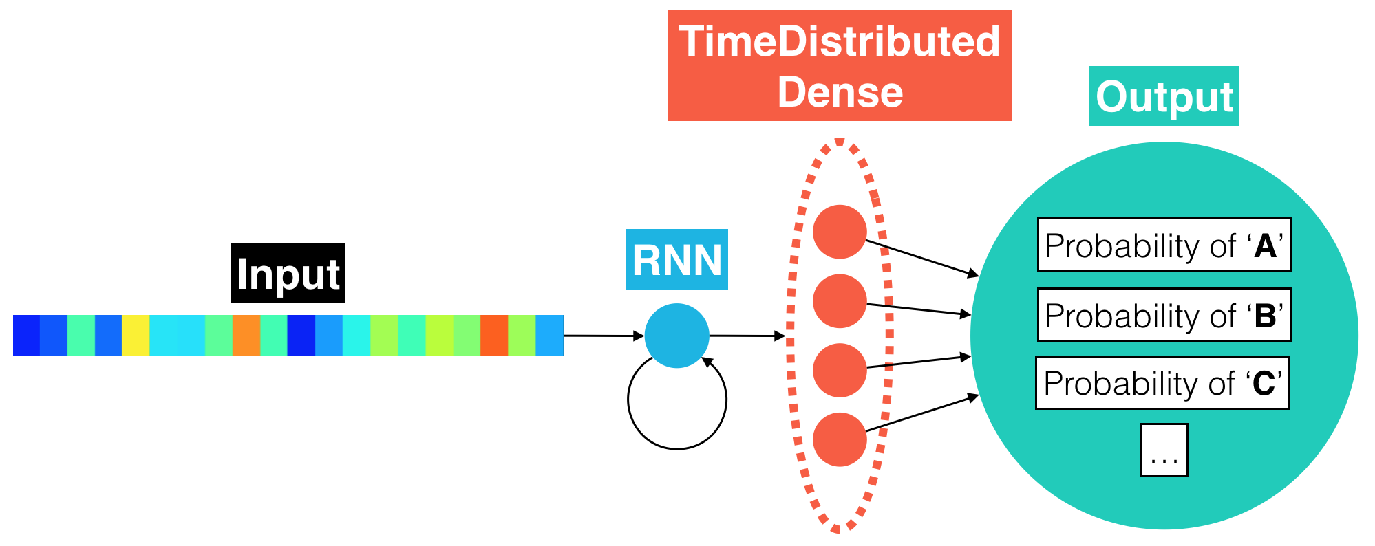
Use your research to complete the rnn_model function within the sample_models.py file. The function should specify an architecture that satisfies the following requirements:
- The first layer of the neural network should be an RNN (
SimpleRNN,LSTM, orGRU) that takes the time sequence of audio features as input. We have addedGRUunits for you, but feel free to changeGRUtoSimpleRNNorLSTM, if you like! - Whereas the architecture in
simple_rnn_modeltreated the RNN output as the final layer of the model, you will use the output of your RNN as a hidden layer. UseTimeDistributedto apply aDenselayer to each of the time steps in the RNN output. Ensure that eachDenselayer hasoutput_dimunits.
Use the code cell below to load your model into the model_1 variable. Use a value for input_dim that matches your chosen audio features, and feel free to change the values for units and activation to tweak the behavior of your recurrent layer.
model_1 = rnn_model(input_dim=161, # change to 13 if you would like to use MFCC features
                    units=200,
                    activation='relu')
Please execute the code cell below to train the neural network you specified in input_to_softmax. After the model has finished training, the model is saved in the HDF5 file model_1.h5. The loss history is saved in model_1.pickle. You are welcome to tweak any of the optional parameters while calling the train_model function, but this is not required.
train_model(input_to_softmax=model_1,
            pickle_path='model_1.pickle',
            save_model_path='model_1.h5',
            spectrogram=True) # change to False if you would like to use MFCC features
(IMPLEMENTATION) Model 2: CNN + RNN + TimeDistributed Dense
The architecture in cnn_rnn_model adds an additional level of complexity, by introducing a 1D convolution layer.
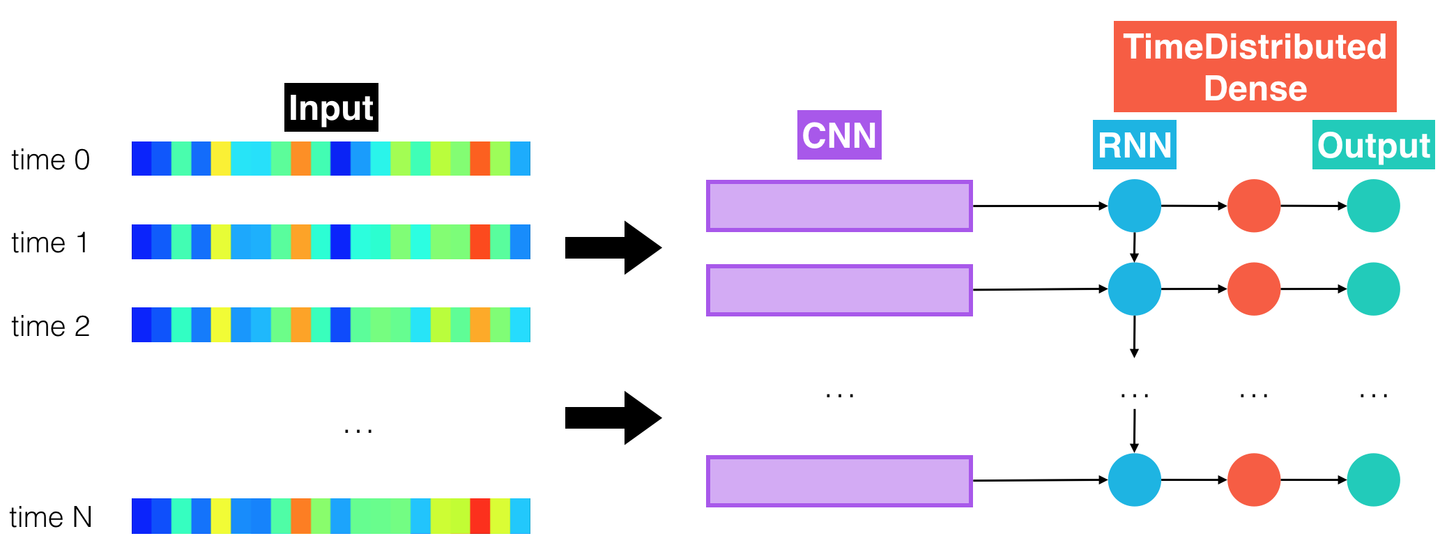
This layer incorporates many arguments that can be (optionally) tuned when calling the cnn_rnn_model module. We provide sample starting parameters, which you might find useful if you choose to use spectrogram audio features.
If you instead want to use MFCC features, these arguments will have to be tuned. Note that the current architecture only supports values of 'same' or 'valid' for the conv_border_mode argument.
When tuning the parameters, be careful not to choose settings that make the convolutional layer overly small. If the temporal length of the CNN layer is shorter than the length of the transcribed text label, your code will throw an error.
Before running the code cell below, you must modify the cnn_rnn_model function in sample_models.py. Please add batch normalization to the recurrent layer, and provide the same TimeDistributed layer as before.
model_2 = cnn_rnn_model(input_dim=161, # change to 13 if you would like to use MFCC features
                        filters=200,
                        kernel_size=11,
                        conv_stride=2,
                        conv_border_mode='valid',
                        units=200)
Please execute the code cell below to train the neural network you specified in input_to_softmax. After the model has finished training, the model is saved in the HDF5 file model_2.h5. The loss history is saved in model_2.pickle. You are welcome to tweak any of the optional parameters while calling the train_model function, but this is not required.
train_model(input_to_softmax=model_2,
            pickle_path='model_2.pickle',
            save_model_path='model_2.h5',
            spectrogram=True) # change to False if you would like to use MFCC features
(IMPLEMENTATION) Model 3: Deeper RNN + TimeDistributed Dense
Review the code in rnn_model, which makes use of a single recurrent layer. Now, specify an architecture in deep_rnn_model that utilizes a variable number recur_layers of recurrent layers. The figure below shows the architecture that should be returned if recur_layers=2. In the figure, the output sequence of the first recurrent layer is used as input for the next recurrent layer.
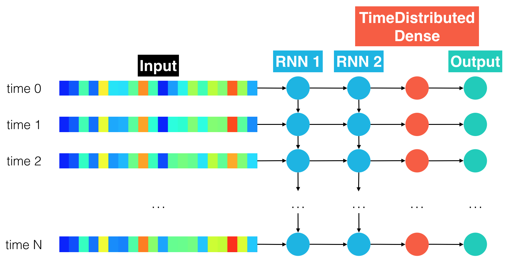
Feel free to change the supplied values of units to whatever you think performs best. You can change the value of recur_layers, as long as your final value is greater than 1. (As a quick check that you have implemented the additional functionality in deep_rnn_model correctly, make sure that the architecture that you specify here is identical to rnn_model if recur_layers=1.)
model_3 = deep_rnn_model(input_dim=161, # change to 13 if you would like to use MFCC features
                         units=200,
                         recur_layers=2)
Please execute the code cell below to train the neural network you specified in input_to_softmax. After the model has finished training, the model is saved in the HDF5 file model_3.h5. The loss history is saved in model_3.pickle. You are welcome to tweak any of the optional parameters while calling the train_model function, but this is not required.
train_model(input_to_softmax=model_3,
            pickle_path='model_3.pickle',
            save_model_path='model_3.h5',
            spectrogram=True) # change to False if you would like to use MFCC features
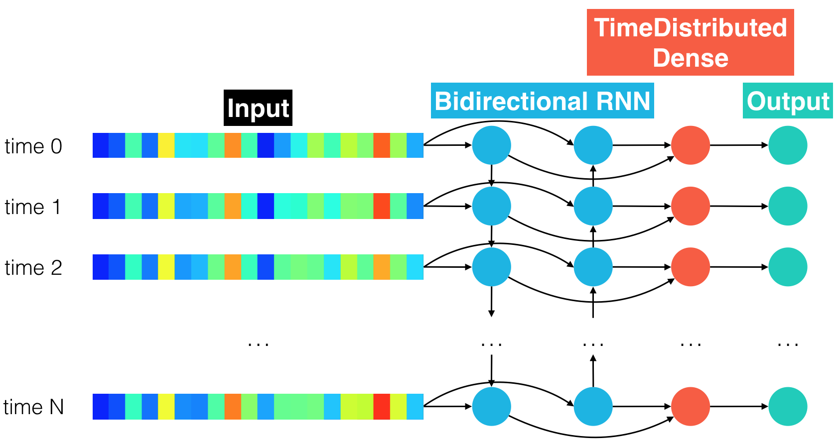
(IMPLEMENTATION) Model 4: Bidirectional RNN + TimeDistributed Dense
Read about the Bidirectional wrapper in the Keras documentation. For your next architecture, you will specify an architecture that uses a single bidirectional RNN layer, before a (TimeDistributed) dense layer. The added value of a bidirectional RNN is described well in this paper.
One shortcoming of conventional RNNs is that they are only able to make use of previous context. In speech recognition, where whole utterances are transcribed at once, there is no reason not to exploit future context as well. Bidirectional RNNs (BRNNs) do this by processing the data in both directions with two separate hidden layers which are then fed forwards to the same output layer.
Before running the code cell below, you must complete the bidirectional_rnn_model function in sample_models.py. Feel free to use SimpleRNN, LSTM, or GRU units. When specifying the Bidirectional wrapper, use merge_mode='concat'.
model_4 = bidirectional_rnn_model(input_dim=161, # change to 13 if you would like to use MFCC features
                                  units=200)
Please execute the code cell below to train the neural network you specified in input_to_softmax. After the model has finished training, the model is saved in the HDF5 file model_4.h5. The loss history is saved in model_4.pickle. You are welcome to tweak any of the optional parameters while calling the train_model function, but this is not required.
train_model(input_to_softmax=model_4,
            pickle_path='model_4.pickle',
            save_model_path='model_4.h5',
            spectrogram=True) # change to False if you would like to use MFCC features
(OPTIONAL IMPLEMENTATION) Models 5+
If you would like to try out more architectures than the ones above, please use the code cell below. Please continue to follow the same convention for saving the models; for the $i$-th sample model, please save the loss at model_i.pickle and saving the trained model at model_i.h5.
## (Optional) TODO: Try out some more models!
### Feel free to use as many code cells as needed.
Compare the Models
Execute the code cell below to evaluate the performance of the drafted deep learning models. The training and validation loss are plotted for each model.
from glob import glob
import numpy as np
import _pickle as pickle
import seaborn as sns
import matplotlib.pyplot as plt
%matplotlib inline
sns.set_style(style='white')

# obtain the paths for the saved model history
all_pickles = sorted(glob("results/*.pickle"))
# extract the name of each model
model_names = [item[8:-7] for item in all_pickles]
# extract the loss history for each model
valid_loss = [pickle.load( open( i, "rb" ) )['val_loss'] for i in all_pickles]
train_loss = [pickle.load( open( i, "rb" ) )['loss'] for i in all_pickles]
# save the number of epochs used to train each model
num_epochs = [len(valid_loss[i]) for i in range(len(valid_loss))]

fig = plt.figure(figsize=(16,5))

# plot the training loss vs. epoch for each model
ax1 = fig.add_subplot(121)
for i in range(len(all_pickles)):
    ax1.plot(np.linspace(1, num_epochs[i], num_epochs[i]),
            train_loss[i], label=model_names[i])
# clean up the plot
ax1.legend()
ax1.set_xlim([1, max(num_epochs)])
plt.xlabel('Epoch')
plt.ylabel('Training Loss')

# plot the validation loss vs. epoch for each model
ax2 = fig.add_subplot(122)
for i in range(len(all_pickles)):
    ax2.plot(np.linspace(1, num_epochs[i], num_epochs[i]),
            valid_loss[i], label=model_names[i])
# clean up the plot
ax2.legend()
ax2.set_xlim([1, max(num_epochs)])
plt.xlabel('Epoch')
plt.ylabel('Validation Loss')
plt.show()

Question 1: Use the plot above to analyze the performance of each of the attempted architectures. Which performs best? Provide an explanation regarding why you think some models perform better than others.
Answer:
Comparing Models
| Model-Name | # of parameters | Architecure | Training Loss | Validation Loss | Category |
|---|---|---|---|---|---|
| Model 0 | 16,617 | RNN | 752.3071 | 722.2373 | Under-fit |
| Model 1 | 223,829 | RNN + TimeDistributed | 128.6848 | 142.4832 | Good-fit |
| Model 2 | 442,029 | CNN + RNN + TimeDistributed | 76.3312 | 139.0822 | Over-fit |
| Model 3 | 465,229 | RNN + RNN + TimeDistributed | 122.3033 | 132.9569 | Good-fit |
| Model 4 | 446,029 | Bi-RNN + TimeDistributed | 103.9919 | 129.1036 | Good-fit |
- Model 0 is underfitting because both its training loss and its validation loss are so high.
- Model 1 is a good fit because its validation loss is relatively close to its training loss.
- Model 2 has the lowest tarining loss. Model 2 is overfitting because its validation loss is much larger than its training loss.CNN is feed-forward network assumes no input structure, thus adding CNN to our network to train a sequential data may be the reason for overfitting.
- Model 3 is a good fit because its validation loss is relatively close to its training loss. RNN exploits sequential data so adding one more RNN instead of CNN to our architecture results a good-fit model.
- Model 4 is a good fit because its validation loss is relatively close to its training loss. Standard recurrent neural network (RNNs) have restrictions as the future input information cannot be reached from the current state. On the contrary, Bi-RNNs do not require their input data to be fixed. Moreover, their future input information is reachable from the current state. The basic idea of BRNNs is to connect two hidden layers of opposite directions to the same output. By this structure, the output layer can get information from past and future states.For this reason Bi-RNN performs better than adding two RNNs to the architecture.(https://en.wikipedia.org/wiki/Bidirectional_recurrent_neural_networks)
(IMPLEMENTATION) Final Model
Now that you've tried out many sample models, use what you've learned to draft your own architecture! While your final acoustic model should not be identical to any of the architectures explored above, you are welcome to merely combine the explored layers above into a deeper architecture. It is NOT necessary to include new layer types that were not explored in the notebook.
However, if you would like some ideas for even more layer types, check out these ideas for some additional, optional extensions to your model:
- If you notice your model is overfitting to the training dataset, consider adding dropout! To add dropout to recurrent layers, pay special attention to the
dropout_Wanddropout_Uarguments. This paper may also provide some interesting theoretical background. - If you choose to include a convolutional layer in your model, you may get better results by working with dilated convolutions. If you choose to use dilated convolutions, make sure that you are able to accurately calculate the length of the acoustic model's output in the
model.output_lengthlambda function. You can read more about dilated convolutions in Google's WaveNet paper. For an example of a speech-to-text system that makes use of dilated convolutions, check out this GitHub repository. You can work with dilated convolutions in Keras by paying special attention to thepaddingargument when you specify a convolutional layer. - If your model makes use of convolutional layers, why not also experiment with adding max pooling? Check out this paper for example architecture that makes use of max pooling in an acoustic model.
- So far, you have experimented with a single bidirectional RNN layer. Consider stacking the bidirectional layers, to produce a deep bidirectional RNN!
All models that you specify in this repository should have output_length defined as an attribute. This attribute is a lambda function that maps the (temporal) length of the input acoustic features to the (temporal) length of the output softmax layer. This function is used in the computation of CTC loss; to see this, look at the add_ctc_loss function in train_utils.py. To see where the output_length attribute is defined for the models in the code, take a look at the sample_models.py file. You will notice this line of code within most models:
model.output_length = lambda x: xThe acoustic model that incorporates a convolutional layer (cnn_rnn_model) has a line that is a bit different:
model.output_length = lambda x: cnn_output_length(
        x, kernel_size, conv_border_mode, conv_stride)
In the case of models that use purely recurrent layers, the lambda function is the identity function, as the recurrent layers do not modify the (temporal) length of their input tensors. However, convolutional layers are more complicated and require a specialized function (cnn_output_length in sample_models.py) to determine the temporal length of their output.
You will have to add the output_length attribute to your final model before running the code cell below. Feel free to use the cnn_output_length function, if it suits your model.
# specify the model
model_end = final_model(input_dim=161,
                        filters=200,
                        kernel_size=11,
                        conv_stride=2,
                        conv_border_mode="valid",
                        units=200,
                        recur_layers=2)
Please execute the code cell below to train the neural network you specified in input_to_softmax. After the model has finished training, the model is saved in the HDF5 file model_end.h5. The loss history is saved in model_end.pickle. You are welcome to tweak any of the optional parameters while calling the train_model function, but this is not required.
train_model(input_to_softmax=model_end,
            pickle_path='model_end.pickle',
            save_model_path='model_end.h5',
            spectrogram=True) # change to False if you would like to use MFCC features
Question 2: Describe your final model architecture and your reasoning at each step.
Answer:
I used Bi-directional RNN because it seems promising in the ASR, because we want to take advantage of previous context.
For each of the Bi-directional RNN layer, I add a batch-normalization layer to speed up the training process.
I add the TimeDistributed layer at the end to better extract complex pattern.
I added drop-out layers for my model not to overfit because we used one Bi-directional RNN in model 4 and validation loss starts to increase from epoch 19 to 20. I think Multiple Bi-directional RNN would cause more if we don't use drop-out layers.
STEP 3: Obtain Predictions
We have written a function for you to decode the predictions of your acoustic model. To use the function, please execute the code cell below.
import numpy as np
from data_generator import AudioGenerator
from keras import backend as K
from utils import int_sequence_to_text
from IPython.display import Audio

def get_predictions(index, partition, input_to_softmax, model_path):
    """ Print a model's decoded predictions
    Params:
        index (int): The example you would like to visualize
        partition (str): One of 'train' or 'validation'
        input_to_softmax (Model): The acoustic model
        model_path (str): Path to saved acoustic model's weights
    """
    # load the train and test data
    data_gen = AudioGenerator()
    data_gen.load_train_data()
    data_gen.load_validation_data()

    # obtain the true transcription and the audio features
    if partition == 'validation':
        transcr = data_gen.valid_texts[index]
        audio_path = data_gen.valid_audio_paths[index]
        data_point = data_gen.normalize(data_gen.featurize(audio_path))
    elif partition == 'train':
        transcr = data_gen.train_texts[index]
        audio_path = data_gen.train_audio_paths[index]
        data_point = data_gen.normalize(data_gen.featurize(audio_path))
    else:
        raise Exception('Invalid partition!  Must be "train" or "validation"')

    # obtain and decode the acoustic model's predictions
    input_to_softmax.load_weights(model_path)
    prediction = input_to_softmax.predict(np.expand_dims(data_point, axis=0))
    output_length = [input_to_softmax.output_length(data_point.shape[0])]
    pred_ints = (K.eval(K.ctc_decode(
                prediction, output_length)[0][0])+1).flatten().tolist()

    # play the audio file, and display the true and predicted transcriptions
    print('-'*80)
    Audio(audio_path)
    print('True transcription:\n' + '\n' + transcr)
    print('-'*80)
    print('Predicted transcription:\n' + '\n' + ''.join(int_sequence_to_text(pred_ints)))
    print('-'*80)
Use the code cell below to obtain the transcription predicted by your final model for the first example in the training dataset.
get_predictions(index=0,
                partition='train',
                input_to_softmax=final_model(input_dim=161,
                        filters=200,
                        kernel_size=11,
                        conv_stride=2,
                        conv_border_mode="valid",
                        units=200,
                        recur_layers=2),
                model_path='./results/model_end.h5')
Use the next code cell to visualize the model's prediction for the first example in the validation dataset.
get_predictions(index=0,
                partition='validation',
                input_to_softmax=final_model(input_dim=161,
                        filters=200,
                        kernel_size=11,
                        conv_stride=2,
                        conv_border_mode="valid",
                        units=200,
                        recur_layers=2),
                model_path='./results/model_end.h5')
One standard way to improve the results of the decoder is to incorporate a language model. We won't pursue this in the notebook, but you are welcome to do so as an optional extension.
If you are interested in creating models that provide improved transcriptions, you are encouraged to download more data and train bigger, deeper models. But beware - the model will likely take a long while to train. For instance, training this state-of-the-art model would take 3-6 weeks on a single GPU!