Estimation Project
###The Tasks ###
In this project, We are asked to build up an estimator in pieces. The details of steps I took are explained below.
Step 1: Sensor Noise
After choosing scenario 06_NoisySensors, I run the simulation for once to collect noisy sensor data and used logs from config/log/Graph1.txt (GPS X data) and config/log/Graph2.txt (Accelerometer X data) files to calculate sandard deviations.
I used below code to process the logged files to figure out the standard deviation of the the GPS X signal and the IMU Accelerometer X signal.
import numpy as np

# Reading from the logs
gps_x  = np.loadtxt('./config/log/Graph1.txt',delimiter=',',dtype='Float64',skiprows=1)[:,1]
acc_x = np.loadtxt('./config/log/Graph2.txt',delimiter=',',dtype='Float64',skiprows=1)[:,1]

#Calculating standard deviations
gps_x_std  = np.std(gps_x)
print(f'GPS X Std: {gps_x_std}')
acc_x_std = np.std(acc_x)
print(f'Accelerometer X Std: {acc_x_std}')
the results:
GPS X Std: 0.6601210006202937
Accelerometer X Std: 0.48276365150441797
I Plug in my result into the top of config/6_Sensornoise.txt by
setting the values as
MeasuredStdDev_GPSPosXY = 0.660
MeasuredStdDev_AccelXY = 0.482
I thought it would be enough to include up to 3 decimal places for the both deviations to include. If my scnerio didn’t pass I was going to include more decimal places to set the values.
Success criteria: The below prints on the console meaning I met the success criteria.
PASS: ABS(Quad.IMU.AX-0.000000) was less than MeasuredStdDev_AccelXY for 67% of the time
*Step 2: ** *Attitude Estimation
We are looking at the first step to our state estimation: including information from our IMU. In this step, we will be improving the complementary filter-type attitude filter with a better rate gyro attitude integration scheme.
I added Commands += AddGraph1.LogToFile and Commands += AddGraph2.LogToFile to 07_AttitudeEstimation file to collect dat to log files. Then I draw the graphs before and after I made changes required to complete this step. The code I used is below :
import numpy as np
import matplotlib.pyplot as plt

%matplotlib inline
%config InlineBackend.figure_format = 'retina'


# time, Quad.Est.E.Yaw, Quad.Est.E.Pitch, Quad.Est.E.Roll, Quad.Est.E.MaxEuler# time,
graph1 = np.loadtxt('./config/log/Graph1.txt',delimiter=',',dtype='Float64',skiprows=1)

# time, Quad.Est.E.Yaw, Quad.Est.E.Pitch, Quad.Est.E.Roll, Quad.Est.E.MaxEuler
no_code_graph1 = np.loadtxt('./config/log/Graph2.txt',delimiter=',',dtype='Float64',skiprows=1)

def plotErrors(data, title):
    """
    Plots the estimation errors on yaw, pith, roll and max euler
    """
    time = data[:, 0]
    sub_titles = ['Yaw', 'Pitch', 'Roll', 'MaxEuler']

    fig, axes = plt.subplots(2, 2, figsize=[20,10])

    for ax, index, sub_title in zip(axes.flat, range(4), sub_titles):
        values = data[:, index + 1]
        ax.plot(time, values, 'r')
        ax.set_xlabel('Time [s]')
        ax.set_ylabel('Error')
        ax.grid()
        ax.set_title(sub_title)

    plt.suptitle(title, fontsize=24)

plotErrors(no_code_graph1, 'Errors linear approximation')
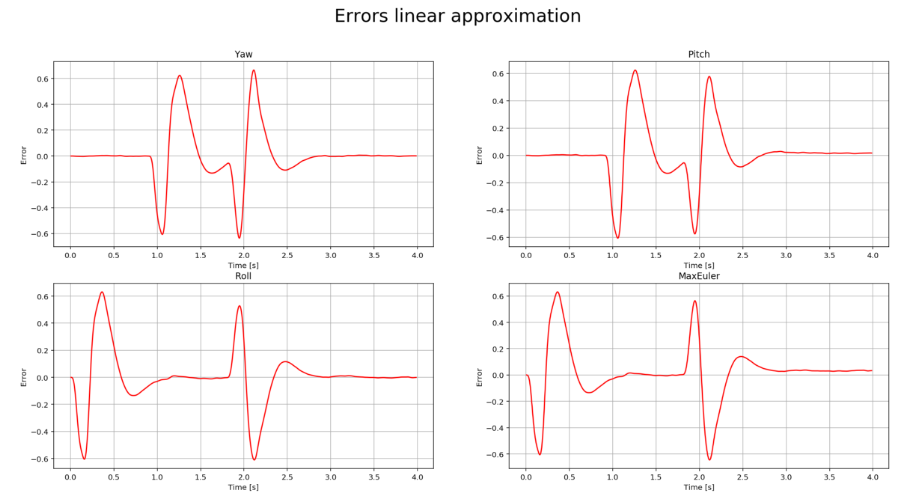 The plots above generated before we made the changes
There are two plots visible in this simulation.
- The top graph is showing errors in each of the estimated Euler angles.
- The bottom shows the true Euler angles and the estimates. Observe that there’s quite a bit of error in attitude estimation.
From QuadEstimatorEKF.cpp file I updated the function UpdateFromIMU() The key difference is I calculated “agle_dot” by adding V3F angle_dot = rot * gyro; line and used it to predict Roll and Pitch instead of using the value come from gyro only.
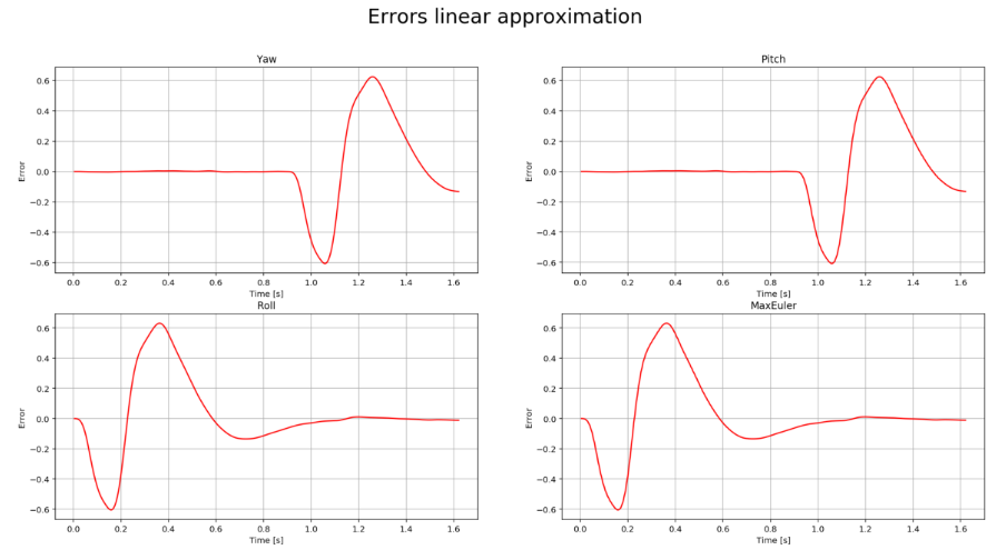 The plots above generated before we made the changes
Success criteria:
The below prints on the console meaning I met the success criteria.
PASS: ABS(Quad.Est.E.MaxEuler) was less than 0.100000 for at least 3.000000 seconds
Step 3: Prediction Step
I also added Commands += AddGraph1.LogToFile and Commands += AddGraph2.LogToFile to 08_PredictState and 09_PredictCovariance file to collect data to log files. Then I draw the graphs before and after I made changes required to complete this step. The code I used is below to plot the logs :
import csv
import numpy as np

import matplotlib.pyplot as plt

%matplotlib inline
%config InlineBackend.figure_format = 'retina'

# time, Quad.Pos.Y, Quad.Est.Y, Quad.Vel.Y, Quad.Est.VY
no_code_graph1 = np.loadtxt('./config/log/Graph1.txt',delimiter=',',dtype='Float64',skiprows=1)
# time, Quad.Pos.Z, Quad.Est.Z, Quad.Vel.Z, Quad.Est.VZ
no_code_graph2 = np.loadtxt('./config/log/Graph2.txt',delimiter=',',dtype='Float64',skiprows=1)

def plotPositionAndVelocity(data,indexPosition, indexVelocity, title):
    """
    Plots the position with index `indexPosition` and the velocity with index `indexVelocity`.
    It assumes the estimations are +1 the index of the values.
    """
    time = data[:, 0]

    trueP = data[:, indexPosition]
    estP = data[:, indexPosition + 1]

    fig, axes = plt.subplots(1, 2, figsize=[20,10])
    axP = axes[0]
    axP.plot(time, trueP - estP, 'r')
    axP.set_xlabel('Time [s]')
    axP.set_ylabel('Error [m]')
    axP.grid()
    axP.set_title('Position')


    trueV = data[:, indexVelocity]
    estV = data[:, indexVelocity + 1]

    axV = axes[1]
    axV.plot(time, (trueV - estV), 'r')
    axV.set_xlabel('Time [s]')
    axV.set_ylabel('Error [m/s]')
    axV.grid()
    axV.set_title('Velocity')

    plt.suptitle(title, fontsize=24)

plotPositionAndVelocity(no_code_graph2, 1, 3, "Z")
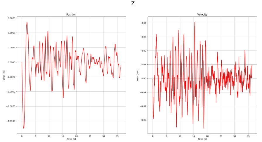 The plot above is generated before we made any changes
After implementing the state prediction step in the PredictState() function.
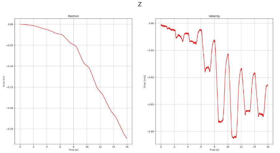 The plot above is generated after we complete PredictState function
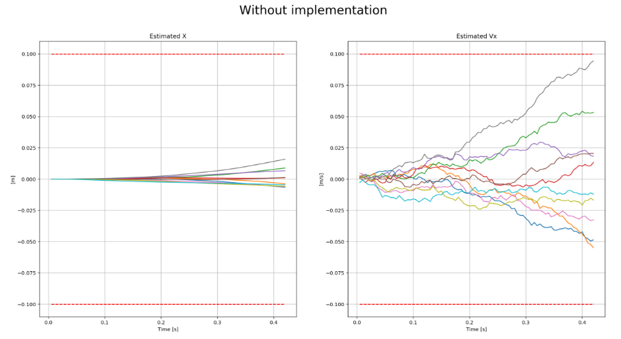 The plot above is generated before we made any changes to GetRgbPrime
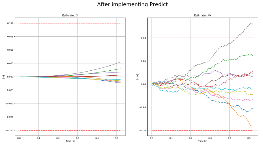 The plot above is generated after we made any changes to GetRgbPrime
Success criteria: This step doesn’t have any specific measurable criteria being checked.
Step 4: Magnetometer Update
I also added Commands += AddGraph1.LogToFile and Commands += AddGraph2.LogToFile to 10_MagUpdate file to collect data to log files. Then I draw the graphs before and after I made changes required to complete this step. The code I used is below to plot the logs :
import numpy as np
import matplotlib.pyplot as plt

%matplotlib inline
%config InlineBackend.figure_format = 'retina'

# time, Quad.MagYaw, Quad.Est.Yaw, Quad.Yaw
no_code_graph1 = np.loadtxt('./config/log/Graph1.txt',delimiter=',',dtype='Float64',skiprows=1)
# time, Quad.Est.E.Yaw, Quad.Est.S.Yaw
no_code_graph2 = np.loadtxt('./config/log/Graph2.txt',delimiter=',',dtype='Float64',skiprows=1)


def  plotYawError(data, title):
    """
    Plots the Yaw error
    """
    time = data[:, 0]
    values = [data[:,1], data[:, 2]]
    subtitles = ['Yaw Error', 'Yaw Std']
    fig, axes = plt.subplots(1, 2, figsize=[20,10])
    for ax, subtitle, value in zip(axes.flat, subtitles, values):
        ax.plot(time, value, 'r')
        ax.set_xlabel('Time [s]')
        ax.set_ylabel('[rad]')
        ax.set_title(subtitle)
        ax.grid()

    plt.suptitle(title, fontsize=24)

plotYawError(no_code_graph2, 'Without modifications')
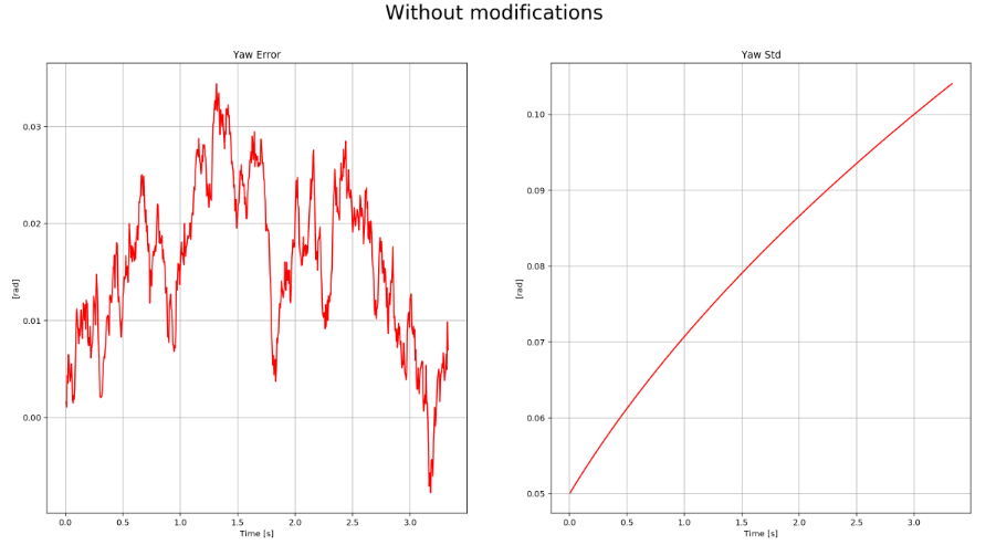 The plot above is generated before we made any changes to UpdareFromMag() function
Before tuning QYawStd parameter fromQuadEstimatorEKF.txt file.
PASS: ABS(Quad.Est.E.Yaw) was less than 0.120000 for at least 10.000000 seconds
FAIL: ABS(Quad.Est.E.Yaw-0.000000) was less than Quad.Est.S.Yaw for 45% of the time
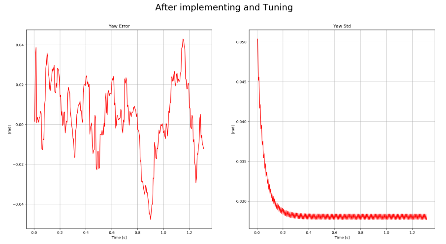 The plot above is generated after we made any changes to UpdareFromMag() function and tuneQYawStd parameter
Success criteria: Below print from the console means I met the success criteria.
PASS: ABS(Quad.Est.E.Yaw) was less than 0.120000 for at least 10.000000 seconds
PASS: ABS(Quad.Est.E.Yaw-0.000000) was less than Quad.Est.S.Yaw for 57% of the time

Step 5: Closed Loop + GPS Update
I also added Commands += AddGraph1.LogToFile and Commands += AddGraph2.LogToFile to 11_GPSUpdate file to collect data to log files. Then I draw the graphs before and after I made changes required to complete this step. The code I used is below to plot the logs :
import numpy as np
import matplotlib.pyplot as plt

%matplotlib inline
%config InlineBackend.figure_format = 'retina'


# time, Quad.Pos.Y, Quad.Est.Y, Quad.Vel.Y, Quad.Est.VY# time,
no_code_graph1 = np.loadtxt('./config/log/Graph1.txt',delimiter=',',dtype='Float64',skiprows=1)
# time, Quad.Est.E.Pos, Quad.Est.S.Z
no_code_graph2 = np.loadtxt('./config/log/Graph2.txt',delimiter=',',dtype='Float64',skiprows=1)


def  plotErrors (data, title):
    """
    Plots the Yaw error
    """
    time = data[:, 0]
    values = [data[:,1], data[:, 2]]
    subtitles = ['Position', 'Std Z']
    fig, axes = plt.subplots(1, 2, figsize=[20,10])
    for ax, subtitle, value in zip(axes.flat, subtitles, values):
        ax.plot(time, value, 'r')
        ax.set_xlabel('Time [s]')
        ax.set_ylabel('[m]')
        ax.set_title(f'{subtitle} - max {np.max(np.absolute(value)):.3f}')
        ax.grid()

    plt.suptitle(title, fontsize=24)

plotErrors(no_code_graph2, 'Without modifications')
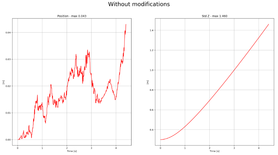 The plot above is generated before we made any changes to config/11_GPSUpdate.tx or update
 UpdateFromGPS() function
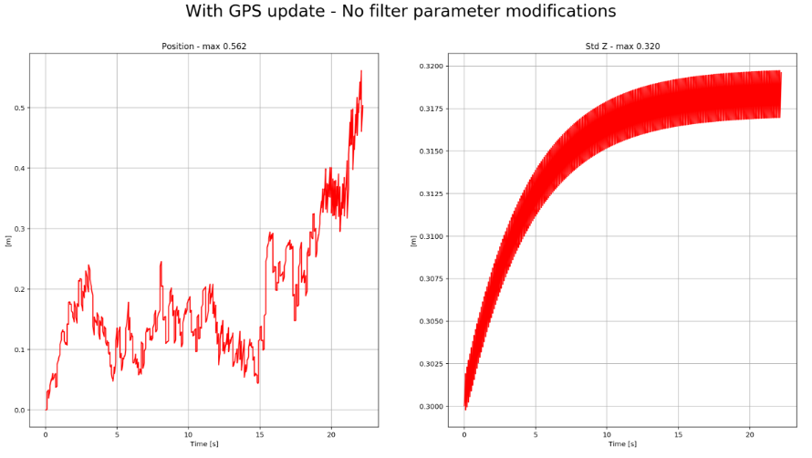 The plot above is generated before we made any changes to config/11_GPSUpdate.tx or update
 UpdateFromGPS() function
Success criteria: Below print from the console means I met the success criteria.
PASS: ABS(Quad.Est.E.Pos) was less than 1.000000 for at least 20.000000 seconds
 Step 6: Adding Your Controller
Changes to the 11_GPSUpdate file and log function is the same function we used at step 5.
After replacing the QuadController.cpp and QuadControlParams.txt files.
The scnerio passes
PASS: ABS(Quad.Est.E.Pos) was less than 1.000000 for at least 20.000000 seconds
Before Tuning:

After Tuning:

Success criteria: Below print from the console means I met the success ciriteria.
PASS: ABS(Quad.Est.E.Pos) was less than 1.000000 for at least 20.000000 seconds